Brush up your NumPy or learn it from scratch

NumPy is a fundamental library that most of the widely used Python data processing libraries are built upon (pandas, OpenCV), inspired by (PyTorch), or can efficiently share data with (TensorFlow, Keras, etc). Understanding how NumPy works gives a boost to your skills in those libraries as well. It is also possible to run NumPy code with no or minimal changes on GPU¹.

The central concept of NumPy is an n-dimensional array. The beauty of it is that most operations look just the same, no matter how many dimensions an array has. But 1D and 2D cases are a bit special. The article consists of three parts:

1. Vectors, the 1D Arrays
2. Matrices, the 2D Arrays
3. 3D and above

I took a great article, “A Visual Intro to NumPy” by Jay Alammar², as a starting point, significantly expanded its coverage, and amended a pair of nuances.

Numpy Array vs. Python List

At first glance, NumPy arrays are similar to Python lists. They both serve as containers with fast item getting and setting and somewhat slower inserts and removals of elements.

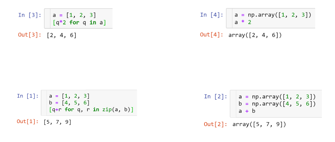
The hands-down simplest example when NumPy arrays beat lists is arithmetic:

Other than that, NumPy arrays are:

• more compact, especially when there’s more than one dimension
• faster than lists when the operation can be vectorized
• slower than lists when you append elements to the end
• usually homogeneous: can only work fast with elements of one type

Here O(N) means that the time necessary to complete the operation is proportional to the size of the array (see Big-O Cheat Sheet³ site), and O*(1) (the so-called “amortized” O(1)) means that the time does not generally depend on the size of the array (see Python Time Complexity⁴ wiki page)

1. Vectors, the 1D Arrays

Vector initialization

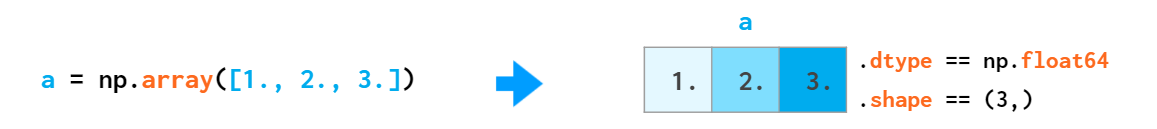
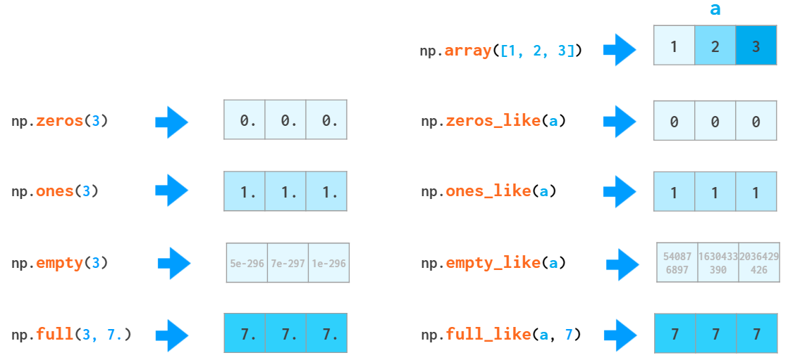
One way to create a NumPy array is to convert a Python list. The type will be auto-deduced from the list element types:

Be sure to feed in a homogeneous list, otherwise you’ll end up with dtype=’object’, which annihilates the speed and only leaves the syntactic sugar contained in NumPy.

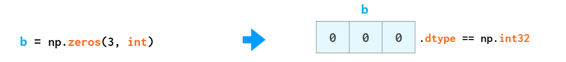
NumPy arrays cannot grow the way a Python list does: No space is reserved at the end of the array to facilitate quick appends. So it is a common practice to either grow a Python list and convert it to a NumPy array when it is ready or to preallocate the necessary space with np.zeros or np.empty:

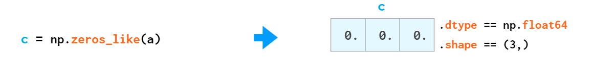
It is often necessary to create an empty array which matches the existing one by shape and elements type:

Actually, all the functions that create an array filled with a constant value have a _like counterpart:

There are as many as two functions for array initialization with a monotonic sequence in NumPy:

If you need a similar-looking array of floats, like [0., 1., 2.], you can change the type of the arange output: arange(3).astype(float), but there’s a better way. The arange function is type-sensitive: If you feed ints as arguments, it will generate ints, and if you feed floats (e.g., arange(3.)) it will generate floats.

But arange is not especially good at handling floats:

This 0.1 looks like a finite decimal number to us but not to the computer: In binary, it is an infinite fraction and has to be rounded somewhere thus an error. That’s why feeding a step with fractional part to arange is generally a bad idea: You might run into an off-by-one error. You can make an end of the interval fall into a non-integer number of steps (solution1) but that reduces readability and maintainability. This is where linspace might come in handy. It is immune to rounding errors and always generates the number of elements you ask for. There’s a common gotcha with linspace, though. It counts points, not intervals, thus the last argument is always plus one to what you would normally think of. So it is 11, not 10 in the example above.

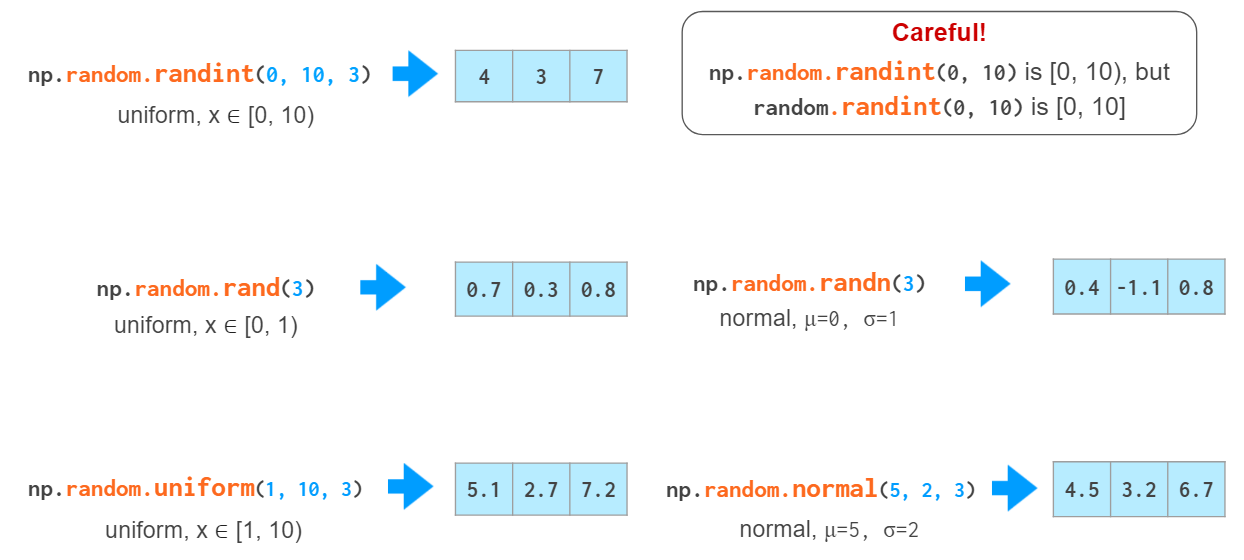
For testing purposes it is often necessary to generate random arrays:

Vector indexing

Once you have your data in the array, NumPy is brilliant at providing easy ways of giving it back:

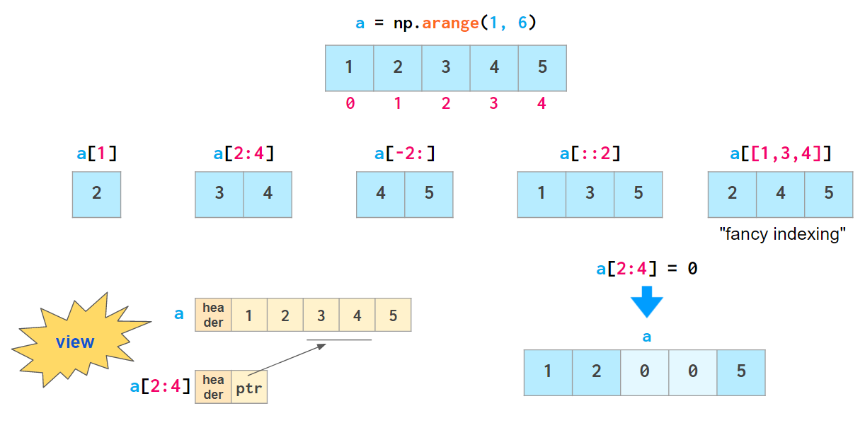
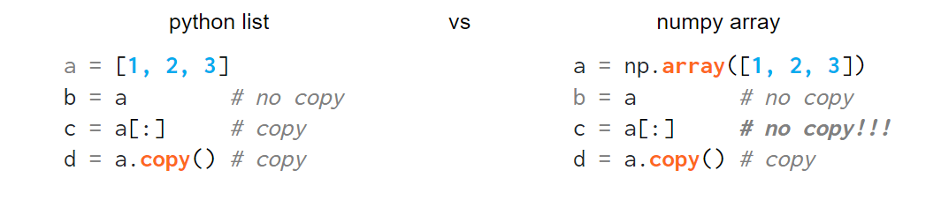
All of the indexing methods presented above except fancy indexing are actually so-called “views”: They don’t store the data and reflect the changes in the original array if it happens to get changed after being indexed.

All of those methods including fancy indexing are mutable: They allow modification of the original array contents through assignment, as shown above. This feature breaks the habit of copying arrays by slicing them:

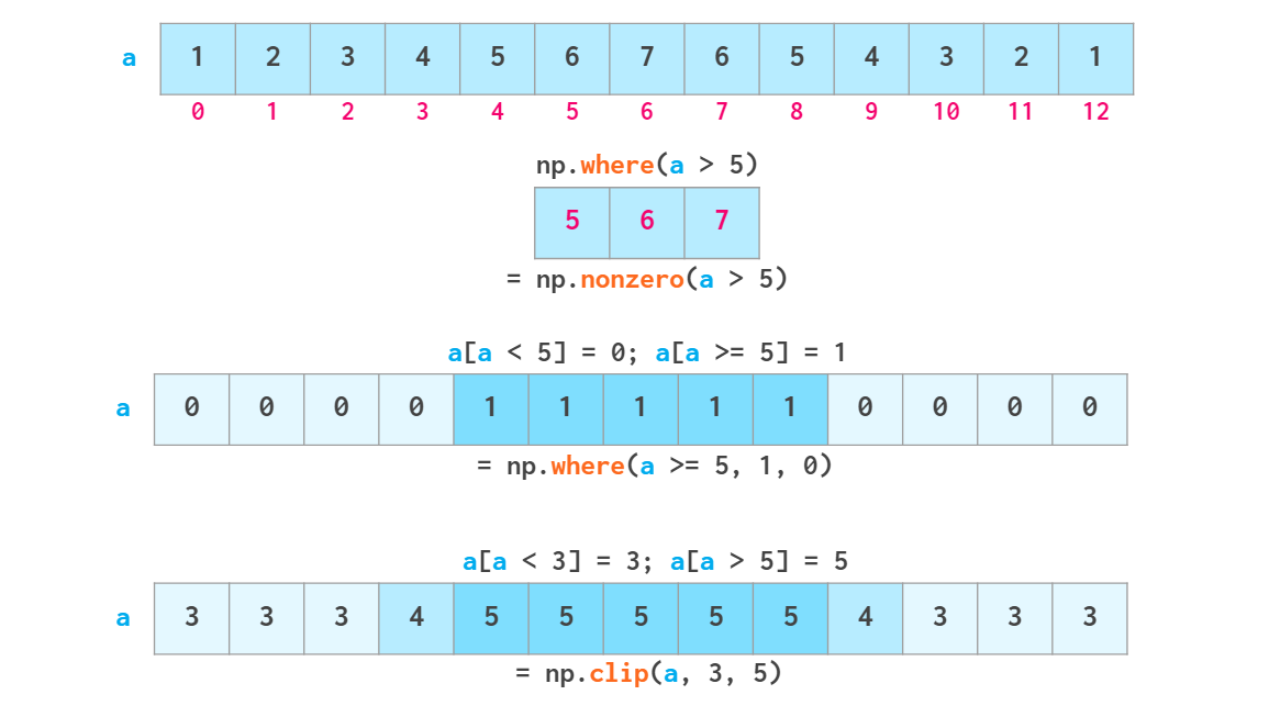
Another super-useful way of getting data from NumPy arrays is boolean indexing, which allows using all kinds of logical operators:

Careful though; Python “ternary” comparisons like 3<=a<=5 don’t work here.

As seen above, boolean indexing is also writable. Two common use cases of it spun off as dedicated functions: the excessively overloaded np.where function (see both meanings below) and np.clip.

Vector operations

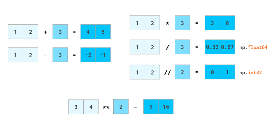
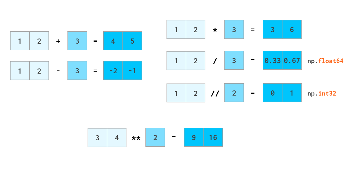
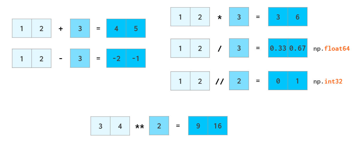
Arithmetic is one of the places where NumPy speed shines most. Vector operators are shifted to the c++ level and allow us to avoid the costs of slow Python loops. NumPy allows the manipulation of whole arrays just like ordinary numbers:

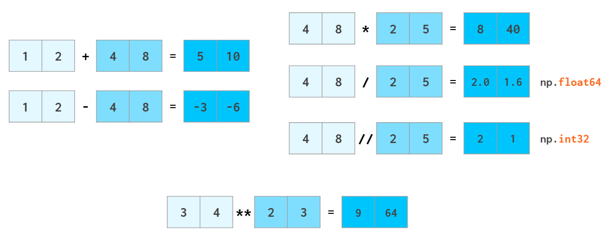
The same way ints are promoted to floats when adding or subtracting, scalars are promoted (aka broadcasted) to arrays:

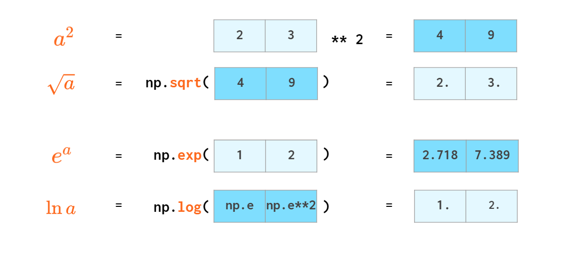
Most of the math functions have NumPy counterparts that can handle vectors:

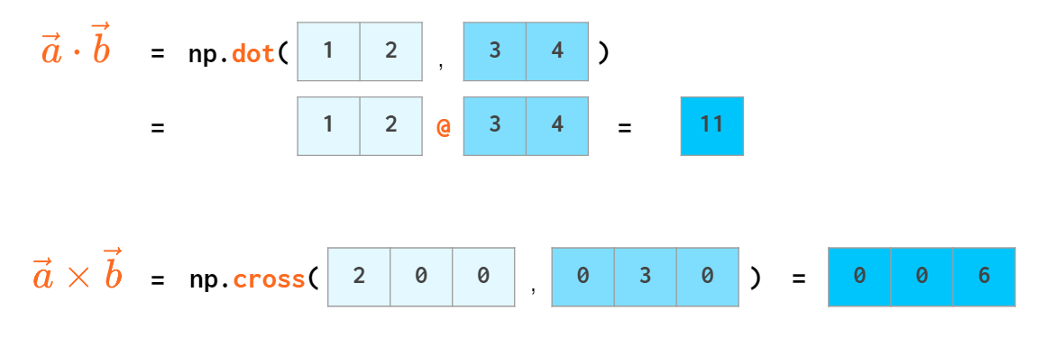
Scalar product has an operator of its own:

You don’t need loops for trigonometry either:

Arrays can be rounded as a whole:

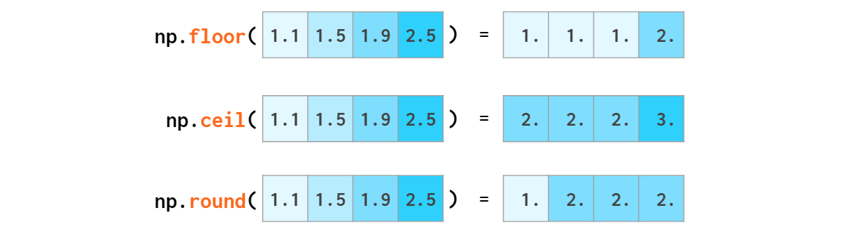
The name np.around is just an alias to np.round introduced to avoid shadowing Python round when you write from numpy import * (as opposed to a more common import numpy as np). You can use a.round() as well.

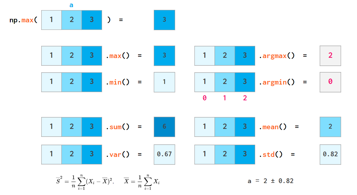
NumPy is also capable of doing the basic stats:

Sorting functions have fewer capabilities than their Python counterparts:

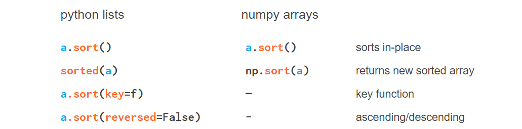
In the 1D case, the absence of the reversed keyword can be easily compensated for by reversing the result. In 2D it is somewhat trickier (feature request⁵).

Searching for an element in a vector

As opposed to Python lists, a NumPy array does not have an index method. The corresponding feature request⁶ has been hanging there for quite a while now.

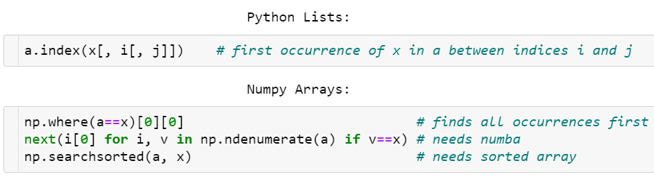
• One way of finding an element is np.where(a==x)[0][0], which is neither elegant nor fast as it needs to look through all elements of the array even if the item to find is in the very beginning.
• A faster way to do it is via accelerating next((i[0] for i, v in np.ndenumerate(a) if v==x), -1) with Numba⁷ (otherwise it’s way slower in the worst case than where).
• Once the array is sorted though, the situation gets better:v = np.searchsorted(a, x); return v if a[v]==x else -1 is really fast with O(log N) complexity, but it requires O(N log N) time to sort first.

Actually, it is not a problem to speed up searching by implementing it in C. The problem is float comparisons. This is a task that simply does not work out of the box for arbitrary data.

Comparing floats

The function np.allclose(a, b) compares arrays of floats with a given tolerance

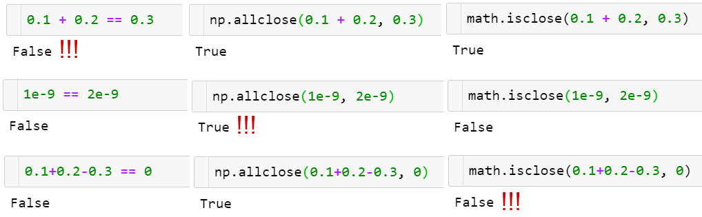
• np.allclose assumes all the compared numbers to be of a typical scale of 1. For example, if you work with nanoseconds, you need to divide the default atol argument value by 1e9: np.allclose(1e-9, 2e-9, atol=1e-17) == False.
• math.isclose makes no assumptions about the numbers to be compared but relies on a user to give a reasonable abs_tol value instead (taking the default np.allclose atol value of 1e-8 is good enough for numbers with a typical scale of 1): math.isclose(0.1+0.2–0.3, abs_tol=1e-8)==True.

Aside from that, np.allclose has some minor issues in a formula for absolute and relative tolerances, for example, for certain a,b allclose(a, b) != allclose(b, a). Those issues were resolved in the (scalar) function math.isclose (which was introduced later). To learn more on that, take a look at the excellent floating-point guide⁸ and the corresponding NumPy issue⁹ on GitHub.

2. Matrices, the 2D Arrays

There used to be a dedicated matrix class in NumPy, but it is deprecated now, so I’ll use the words matrix and 2D array interchangeably.

Matrix initialization syntax is similar to that of vectors:

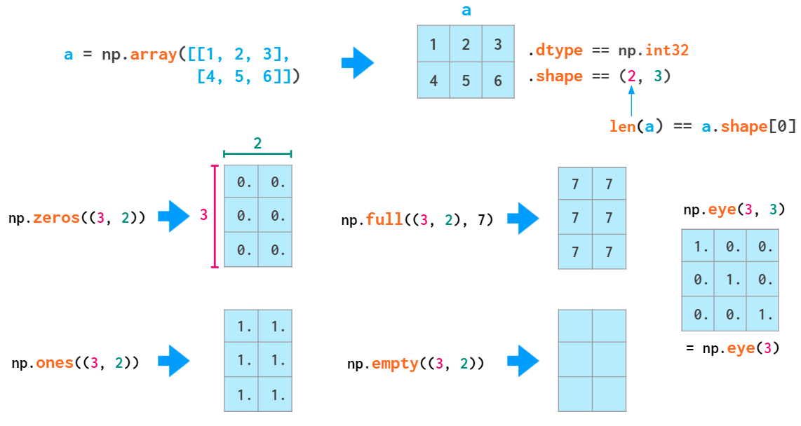
Double parentheses are necessary here because the second positional parameter is reserved for the (optional) dtype (which also accepts integers).

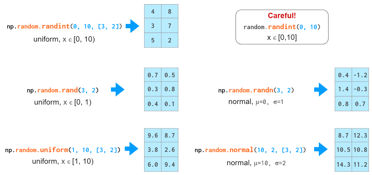
Random matrix generation is also similar to that of vectors:

Two-dimensional indexing syntax is more convenient than that of nested lists:

The “view” sign means that no copying is actually done when slicing an array. When the array is modified, the changes are reflected in the slice as well.

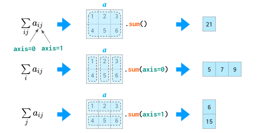
The axis argument

In many operations (e.g., sum) you need to tell NumPy if you want to operate across rows or columns. To have a universal notation that works for an arbitrary number of dimensions, NumPy introduces a notion of axis: The value of the axis argument is, as a matter of fact, the number of the index in question: The first index is axis=0, the second one is axis=1, and so on. So in 2D axis=0 is column-wise andaxis=1 means row-wise.

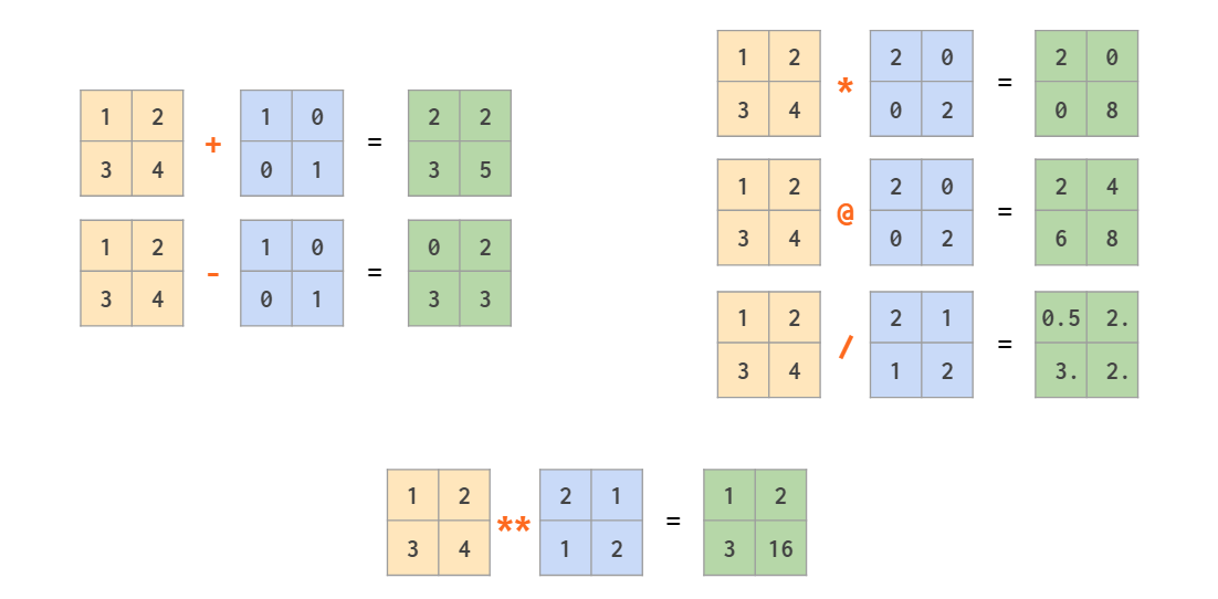
Matrix arithmetic

In addition to ordinary operators (like +,-,*,/,// and **) which work element-wise, there’s a @ operator that calculates a matrix product:

As a generalization of broadcasting from scalar that we’ve seen already in the first part, NumPy allows mixed operations between a vector and a matrix, and even between two vectors:

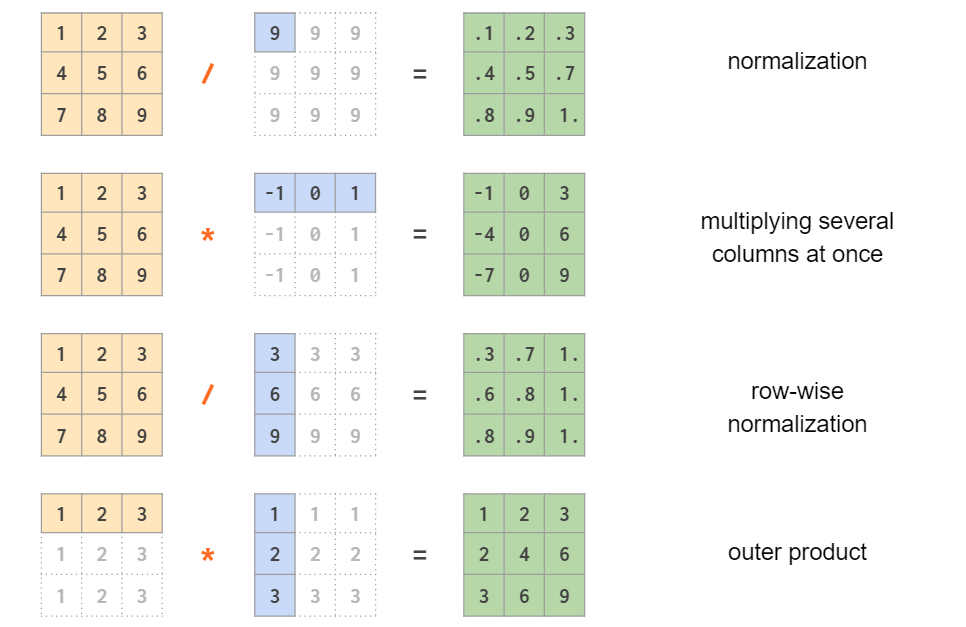
Note that in the last example it is a symmetric per-element multiplication. To calculate the outer product using an asymmetric linear algebra matrix multiplication the order of the operands should be reversed:

Row vectors and column vectors

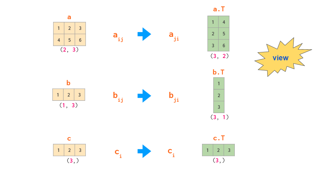
As seen from the example above, in the 2D context, the row and column vectors are treated differently. This contrasts with the usual NumPy practice of having one type of 1D arrays wherever possible (e.g., a[:,j] — the j-th column of a 2D array a— is a 1D array). By default 1D arrays are treated as row vectors in 2D operations, so when multiplying a matrix by a row vector, you can use either shape (n,) or (1, n) — the result will be the same. If you need a column vector, there are a couple of ways to cook it from a 1D array, but surprisingly transpose is not one of them:

Two operations that are capable of making a 2D column vector out of a 1D array are reshaping and indexing with newaxis:

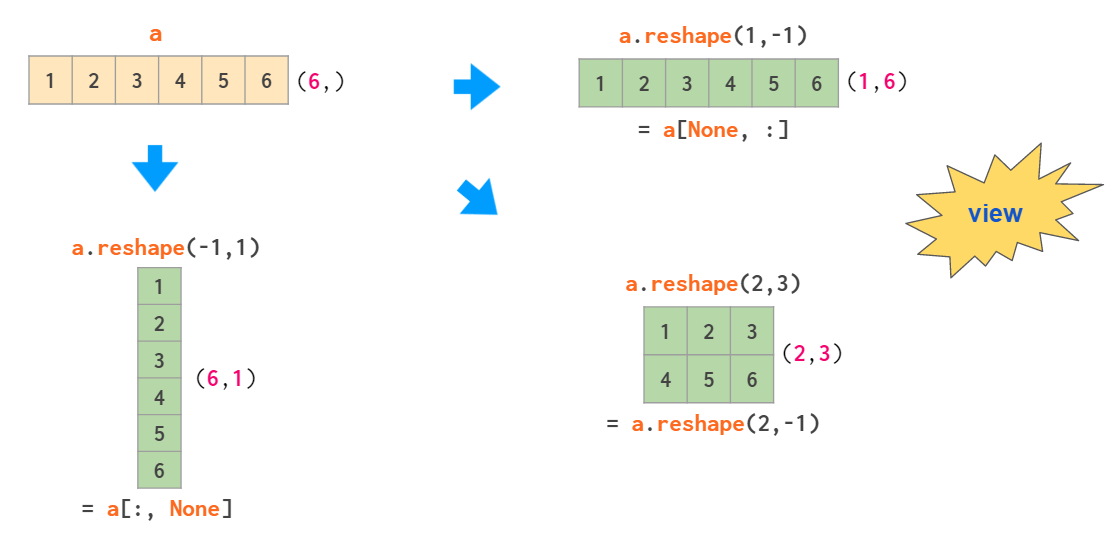
Here the -1 argument tells reshape to calculate one of the dimension sizes automatically and None in the square brackets serves as a shortcut for np.newaxis, which adds an empty axis at the designated place.

So, there’s a total of three types of vectors in NumPy: 1D arrays, 2D row vectors, and 2D column vectors. Here’s a diagram of explicit conversions between those:

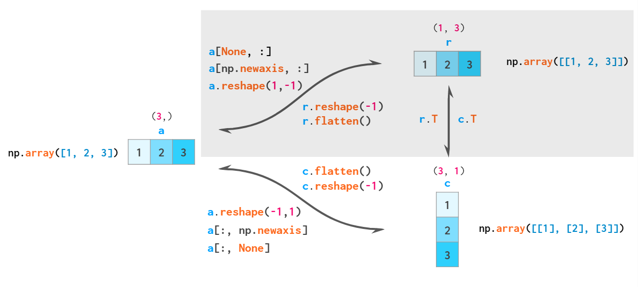
By the rules of broadcasting, 1D arrays are implicitly interpreted as 2D row vectors, so it is generally not necessary to convert between those two — thus the corresponding area is shaded.

Matrix manipulations

There are two main functions for joining the arrays:

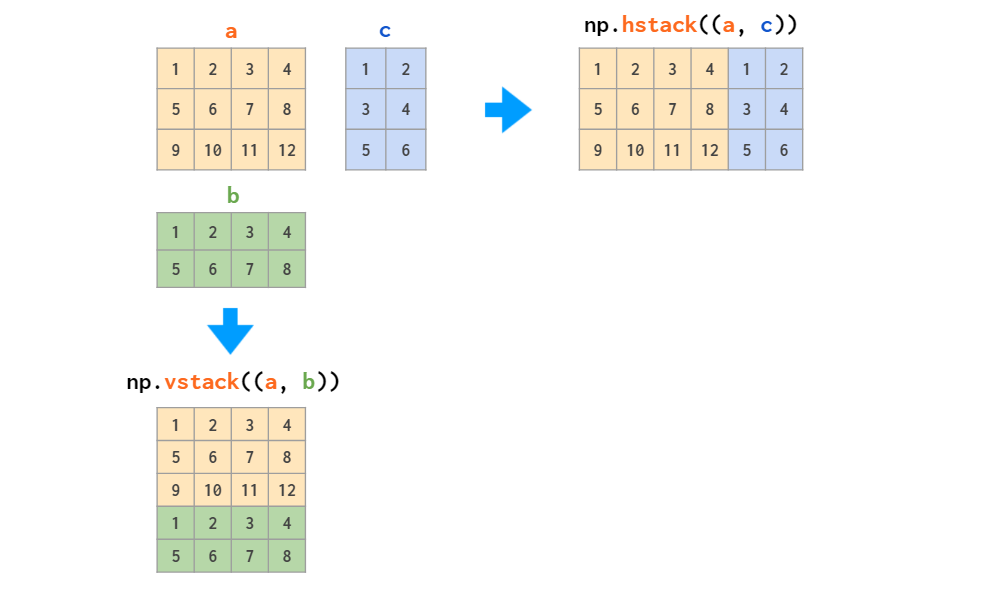
Those two work fine with stacking matrices only or vectors only, but when it comes to mixed stacking of 1D arrays and matrices, only the vstack works as expected: The hstack generates a dimensions-mismatch error because as described above, the 1D array is interpreted as a row vector, not a column vector. The workaround is either to convert it to a row vector or to use a specialized column_stack function which does it automatically:

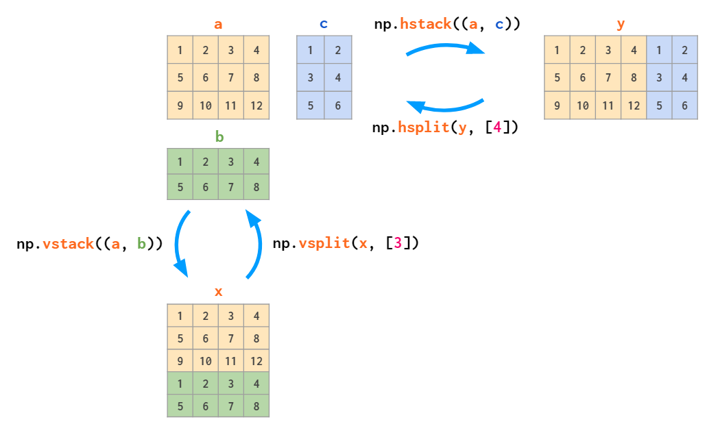
The inverse of stacking is splitting:

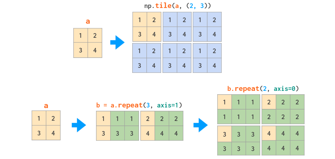
Matrix replication can be done in two ways: tile acts like copy-pasting and repeat like collated printing:

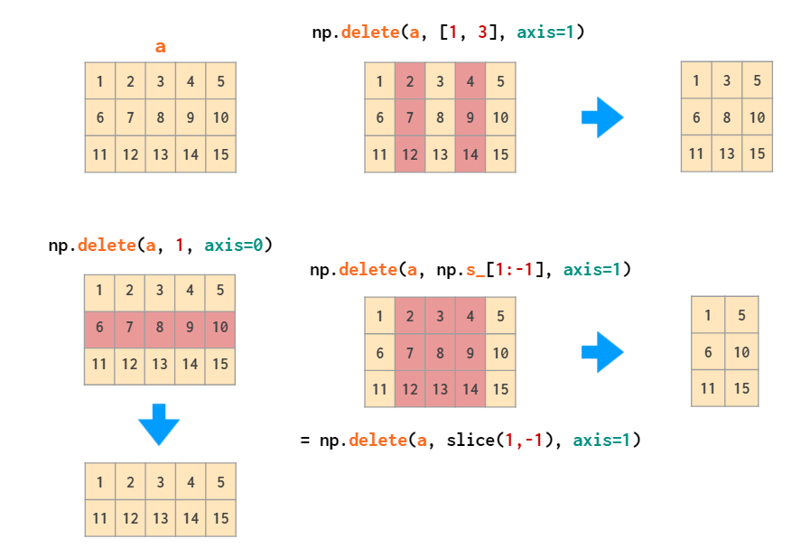
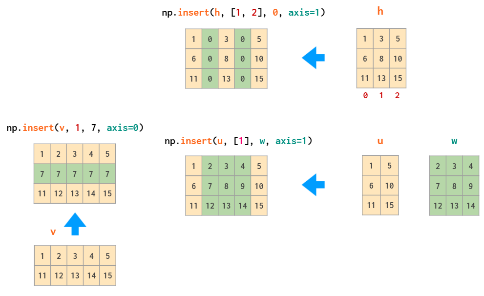
Specific columns and rows can be deleted like that:

The inverse operation is insert:

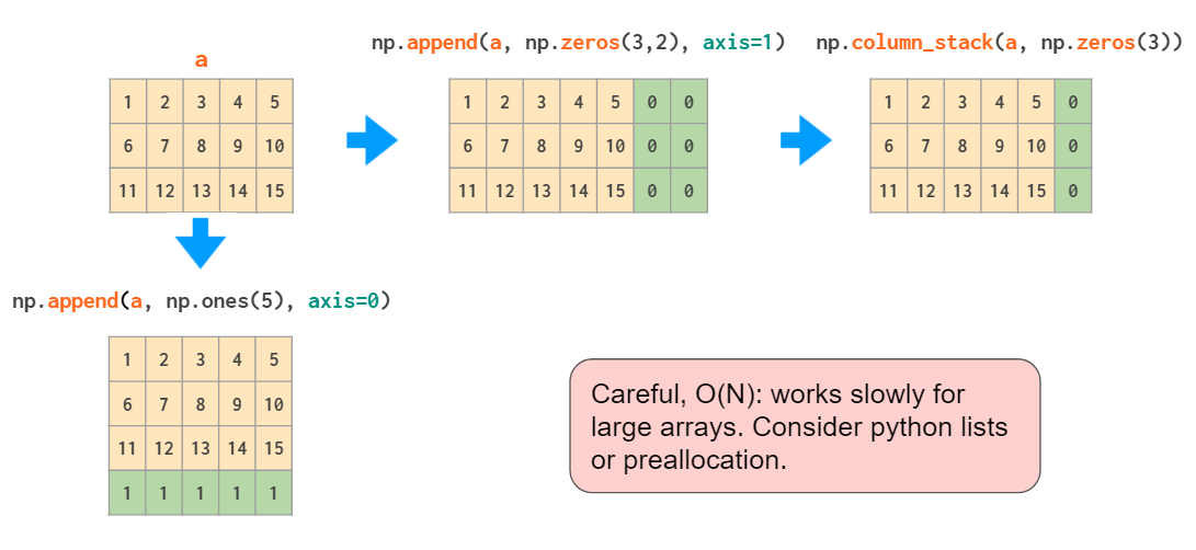
The append function, just like hstack, is unable to automatically transpose 1D arrays, so once again, either the vector needs to be reshaped or a dimension added, or column_stack needs to be used instead:

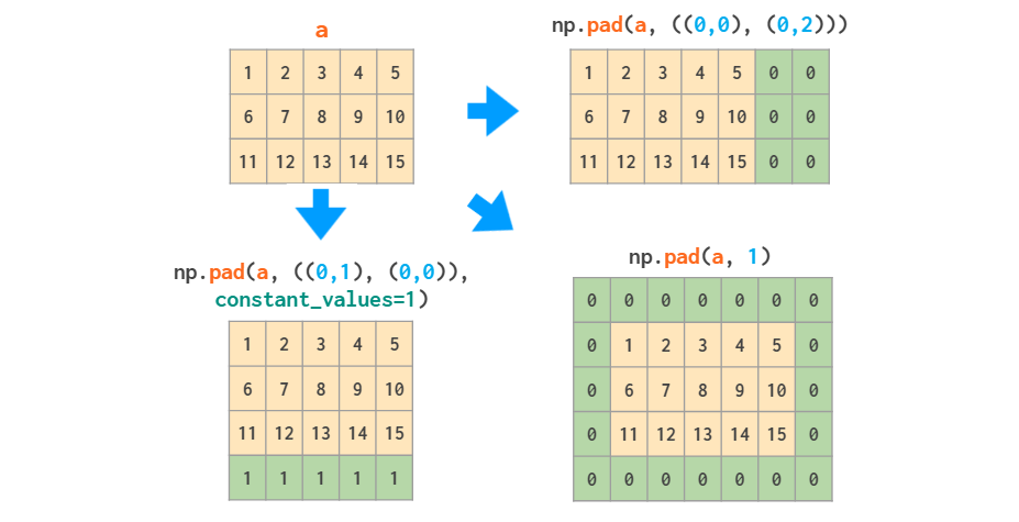
Actually, if all you need to do is add constant values to the border(s) of the array, the (slightly overcomplicated) pad function should suffice:

Meshgrids

The broadcasting rules make it simpler to work with meshgrids. Suppose, you need the following matrix (but of a very large size):

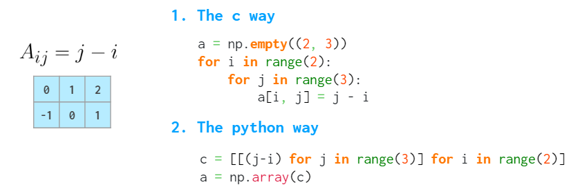
Two obvious approaches are slow, as they use Python loops. The MATLAB way of dealing with such problems is to create a meshgrid:

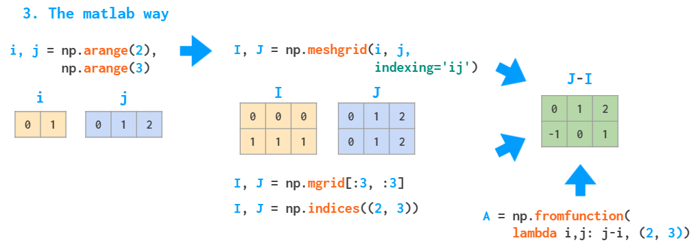
The meshgrid function accepts an arbitrary set of indices, mgrid — just slices and indices can only generate the complete index ranges. fromfunction calls the provided function just once, with the I and J argument as described above.

But actually, there is a better way to do it in NumPy. There’s no need to spend memory on the whole I and J matrices (even though meshgrid is smart enough to only store references to the original vectors if possible). It is sufficient to store only vectors of the correct shape, and the broadcasting rules take care of the rest:

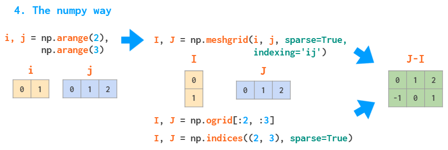
Without the indexing=’ij’ argument, meshgrid will change the order of the arguments: J, I= np.meshgrid(j, i) — it is an ‘xy’ mode, useful for visualizing 3D plots (see the example from the docs).

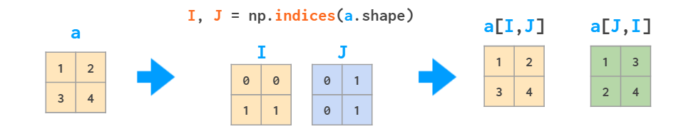
Aside from initializing functions over a two- or three-dimensional grid, the meshes can be useful for indexing arrays:

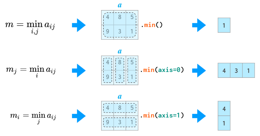
Matrix statistics

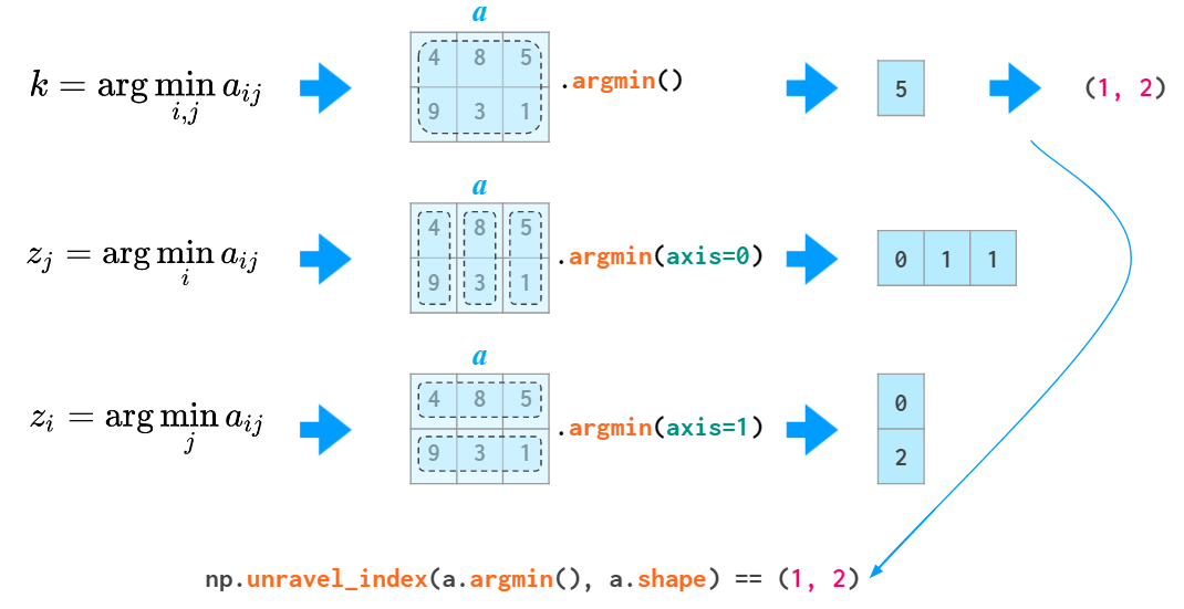
Just like sum, all the other stats functions (min/max, argmin/argmax, mean/median/percentile, std/var) accept the axis parameter and act accordingly:

The argmin and argmax functions in 2D and above have an annoyance of returning the flattened index (of the first instance of the min and max value). To convert it to two coordinates, an unravel_index function is required:

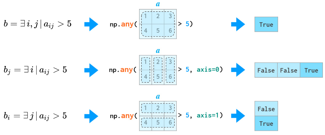
The quantifiers all and any are also aware of the axis argument:

Matrix sorting

As helpful as the axis argument is for the functions listed above, it is as unhelpful for the 2D sorting:

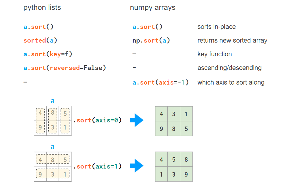
It is just not what you would usually want from sorting a matrix or a spreadsheet: axis is in no way a replacement for the key argument. But luckily, NumPy has several helper functions which allow sorting by a column — or by several columns, if required:

1. a[a[:,0].argsort()] sorts the array by the first column:

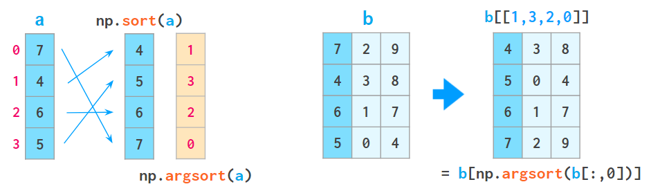
Here argsort returns an array of indices of the original array after sorting.

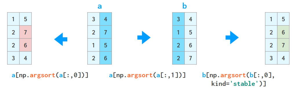
This trick can be repeated, but care must be taken so that the next sort does not mess up the results of the previous one:
a = a[a[:,2].argsort()]
a = a[a[:,1].argsort(kind='stable')]
a = a[a[:,0].argsort(kind='stable')]

2. There’s a helper function lexsort which sorts in the way described above by all available columns, but it always performs row-wise, and the order of rows to be sorted is inverted (i.e., from bottom to top) so its usage is a bit contrived, e.g.
– a[np.lexsort(np.flipud(a[2,5].T))] sorts by column 2 first and then (where the values in column 2 are equal) by column 5.
– a[np.lexsort(np.flipud(a.T))] sorts by all columns in left-to-right order.

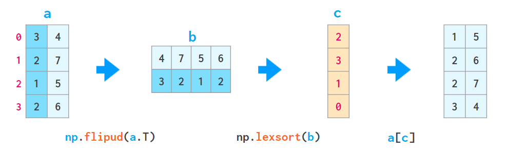
Here flipud flips the matrix in the up-down direction (to be precise, in the axis=0 direction, same as a[::-1,...], where three dots mean “all other dimensions’”— so it’s all of a sudden flipud, not fliplr, that flips the 1D arrays).

3. There also is an order argument to sort, but it is neither fast nor easy to use if you start with an ordinary (unstructured) array.

4. It might be a better option to do it in pandas since this particular operation is way more readable and less error-prone there:
– pd.DataFrame(a).sort_values(by=[2,5]).to_numpy() sorts by column 2, then by column 5.
– pd.DataFrame(a).sort_values().to_numpy() sorts by all columns in the left-to-right order.

3. 3D and Above

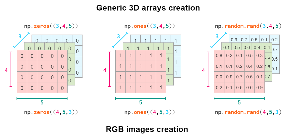
When you create a 3D array by reshaping a 1D vector or converting a nested Python list, the meaning of the indices is (z,y,x). The first index is the number of the plane, then the coordinates go in that plane:

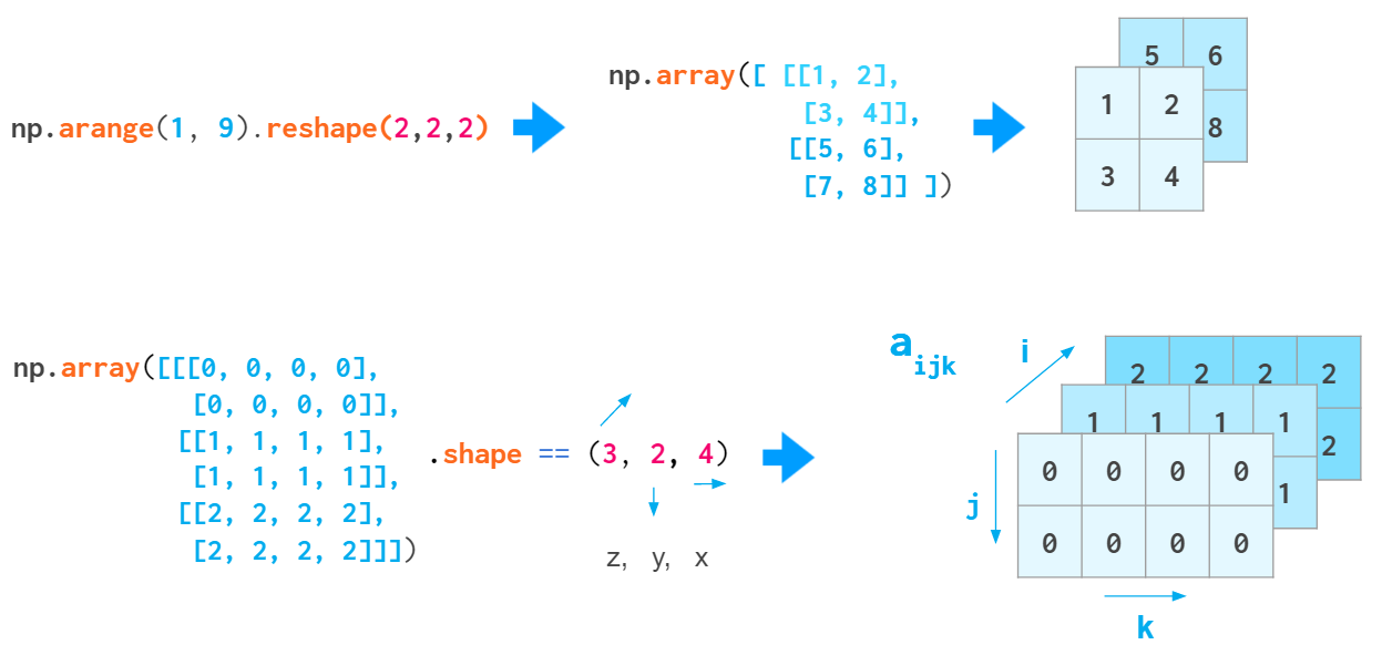
This index order is convenient, for example, for keeping a bunch of gray-scale images: a[i] is a shortcut for referencing the i-th image.

But this index order is not universal. When working with RGB images, the (y,x,z) order is usually used: First are two pixel coordinates, and the last one is the color coordinate (RGB in Matplotlib, BGR in OpenCV):

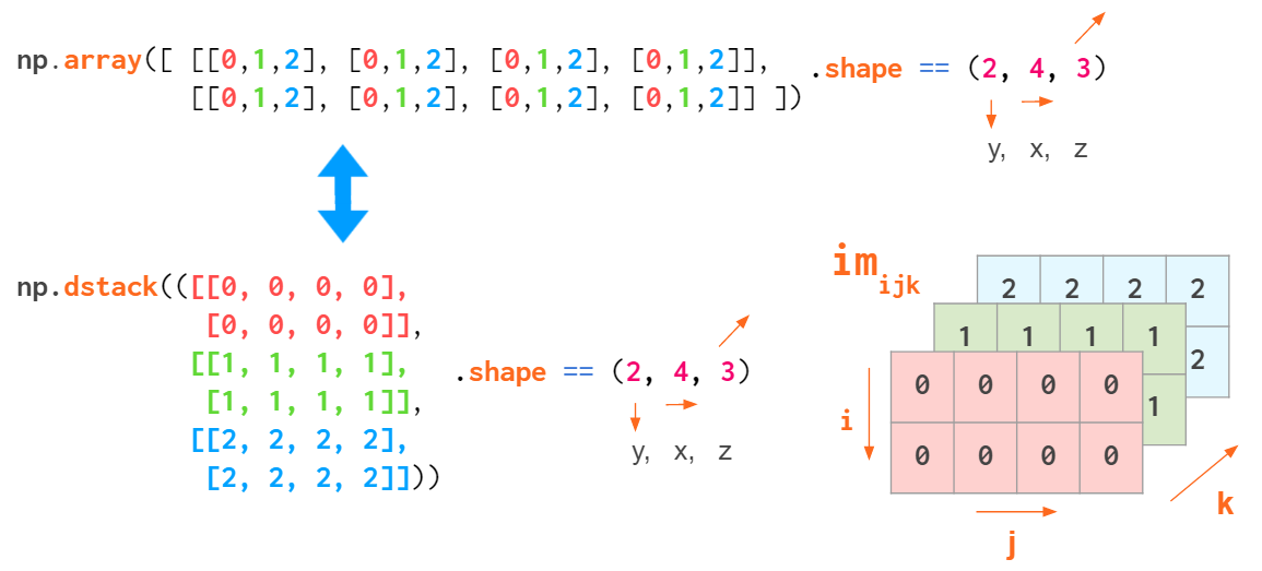
This way it is convenient to reference a specific pixel: a[i,j] gives an RGB tuple of the (i,j) pixel.

So the actual command to create a certain geometrical shape depends on the conventions of the domain you’re working on:

Obviously, NumPy functions like hstack, vstack, or dstack are not aware of those conventions. The index order hardcoded in them is (y,x,z), the RGB images order:

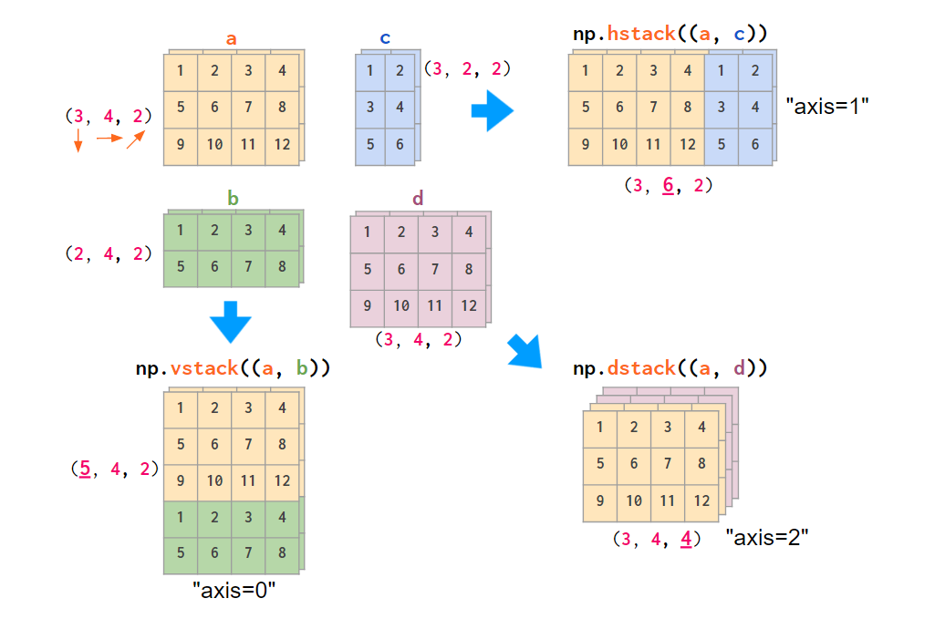
If your data is laid out differently, it is more convenient to stack images using the concatenate command, feeding it the explicit index number in an axis argument:

If thinking in terms of axes numbers is not convenient to you, you can convert the array to the form that is hardcoded into hstack and co:

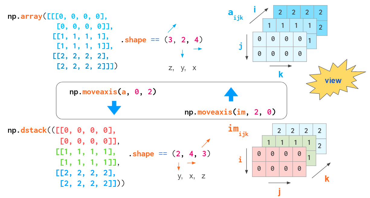
This conversion is cheap: No actual copying takes place; it just mixes the order of indices on the fly.

Another operation that mixes the order of indices is array transposition. Examining it might make you feel more familiar with 3D arrays. Depending on the order of axes you’ve decided on, the actual command to transpose all planes of your array will be different: For generic arrays, it is swapping indices 1 and 2, for RGB images it is 0 and 1:

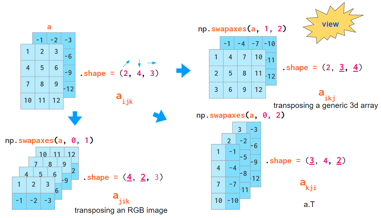
Interesting though that the default axes argument for transpose (as well as the only a.T operation mode) reverses the index order, which coincides with neither of the index order conventions described above.

And finally, here’s a function that can save you a lot of Python loops when dealing with the multidimensional arrays and can make your code cleaner —einsum (Einstein summation):

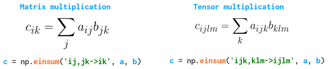
It sums the arrays along the repeated indices. In this particular example np.tensordot(a, b, axis=1) would suffice in both cases, but in the more complex cases einsum might work faster and is generally easier to both write and read — once you understand the logic behind it.

If you want to test your NumPy skills, there’s a tricky crowd-sourced set of 100 NumPy exercises¹⁰ on GitHub.

Let me know (on reddit, hackernews, etc) if I have missed your favorite NumPy feature, and I’ll try to fit it in!

References

1. Scott Sievert, NumPy GPU acceleration
2. Jay Alammar, A Visual Intro to NumPy and Data Representation
3. Big-O Cheat Sheet site
4. Python Time Complexity wiki page
5. NumPy Issue #14989, Reverse param in ordering functions
6. NumPy Issue #2269, First nonzero element
7. Numba library homepage
8. The Floating-Point Guide, Comparison
9. NumPy Issue #10161, numpy.isclose vs math.isclose
10. 100 NumPy exercises on GitHub