The Unreasonable Syntactic Expressivity of RNNs

We prove a result that demonstrates RNNs can exactly implement bounded-depth stacks to capture a building block of human language optimally efficiently. Sit back, relax, grab some popcorn. This is a 24 minute banger.

The Unreasonable Syntactic Expressivity of RNNs

In 2015, Andrej Karpathy posted a now famous blog post on The Unreasonable Effectiveness of Recurrent Neural Networks.¹ In it, he shared some of the wonder he felt at the empirical utility and learning behavior of RNNs. To summarize this sense of wonder, Karpathy emphasized:

We’ll train RNNs to generate text character by character and ponder the question “how is that even possible?”

Re-reading Karpathy’s blog post recently, even in the era of large pre-trained transformers, I still found the effectiveness of modestly sized RNNs for learning highly structured output spaces fascinating. For example, Andrej shows samples from an RNN trained on Wikipedia, which learns to generate not just relatively grammatical English, but Wikipedia article structure and even valid XML code.

In this blog post, we describe a recent step towards understanding Karpathy’s question – how is that even possible?

Prelude: RNNs work, but how?

Empirically, RNNs are pretty effective in learning the syntax of language! On the one hand, to really process hierarchical structure in general, it’s necessary emulate pushing and popping elements from a stack, a fundamental operation in parsing. On the other hand, there’s healthy skepticism about RNNs; they might simply be counting up statistics about likely (long) word sequences like an n-gram model, and sharing some statistical strength due to word embeddings.

So, which is it? The mushy hidden state of an RNN doesn’t seem amenable to stack-like behavior, and many models have been made to make up for this, from the Ordered Neuron variant of the LSTM (Shen et al., 2019) to RNNs augmented with an explicit, external stack (Joulin and Mikolov, 2015). It’s even been proven that RNNs can’t recognize hierarchical languages in general (Merrill et al., 2020)! Things aren’t looking great for the stack story, which helps us clarify our how is that possible question: is stack-like behavior even possible in RNNs in a realistic setting?

We add one insight to this question: when processing natural language, we can bound the maximum number of things we’ll need to store on the stack. Once you assume this, we were very surprised to prove a formal version of the following:

We prove that RNNs can do this, not that they learn to do this. However, our proof consists of explicit mechanisms by which RNNs can implement bounded-depth stacks, in fact, we also provide a separate, more efficient mechanism for LSTMs that solely uses its gates.

Our result changed the way I think about RNNs. It’s true that RNNs can’t implement arbitrary-depth stacks (like a pushdown automaton can). They have finite memory, so they’re finite-state machines). However, they can turn their hidden states into stack structured memory, meaning they can process some (bounded, hierarchical!) languages exponentially more efficiently than one would think if they were learning the finite-state machine. We argue this means the Chomsky Hierarchy isn’t the (only) thing we should be using to characterize neural models’ expressivity; even in the simplest (finite-state) regime, the structure of the memory of these networks is of interest. We hope that our proofs and constructions help people think about and analyze RNN behavior, and inspire future improvements in neural architectures.

This blog post is based off the paper RNNs can generate bounded hierarchical languages with optimal memory, published at EMNLP 2020, joint work with Michael Hahn, Surya Ganguli, Percy Liang, and Chris Manning.

Theoretical tl;dr: we introduce Dyck-$(k,m)$, the language of nested brackets of $k$ types and nesting depth at most $m$, and prove that RNNs can generate these languages in $O\left(m\log k\right)$ hidden units, an exponential improvement over known constructions, which would use $O\left(k^{m/2}\right)$. We also prove that this is tight; using $o\left(m\log k\right)$ is impossible.

Hierarchical structure and language

We’ll start with the second most interesting part of NLP: language². In human languages, the order in which words are spoken matters^{[citation needed]}. But their order doesn’t provide the whole story off the bat; there’s rich structure in human languages that governs how the meanings of words and phrases are composed to form the meanings of larger bits of language. The insufficiency of the linear (that is, “as given”) order of language is clear due to hierarchical dependenices in language. For example, consider the following sentence:

The chef is exceptional.

All’s good so far, but consider the following:

The chef who went to the stores is exceptional.

Here, it’s still the chef that’s exceptional, not the stores, showing that the (chef, is) relationship is not based linear order. We can keep playing this game more or less for as long as we’d like:

The chef who went to the stores and picked up the onions is exceptional.

The subject/verb agreement relationship in English, as with (chef, is), is a nice example of the hierarchical nature of language. More generally, the sentential hierarchical relationships of language are described in syntactic annotation, usually in the form of trees, like in the following phrases³:

The two trees provide two distinct interpretations of the phrase Natural Language Processing. In the leftmost tree, language and processing first combine. Then language processing combines with natural. So, it’s language processing that’s performed or characterized by its naturalness. Is this the intended reading of NLP? I’d argue, no. In the rightmost tree, we have natural combine with language. then natural language combines with processing, meaning we’re processing this thing called natural language. That’s more like it.

A common formalism for syntax is the context-free grammar, both for natural language and for languages like XML. The example we gave above for the phrase Natural Language Processing is informally in constituency form, but here’s a full example⁴:

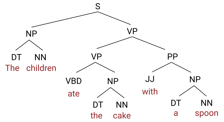
The labels on the tree are very useful, but we won’t go into what they mean here. To see the connection between such a structure and a stack, consider a preorder traversal of the tree.

    (S (NP (DT The ) (NN children)) (VP (VBD ate) (NP (DT the) (NN cake))) (PP (JJ with) (NP (DT a) (NN spoon))))

If one had access to this explicit linear representation of the tree, one could imagine pushing the (S token, then the (NP, then pushing (and popping) the (DT and The and ), and so on, to keep track of what unfinished constituents were under construction. A key difficulty of processing real language, of course, is that the internal nodes (like (S) are not provided; this is why parsing isn’t trivial for natural language. But even with access to these internal nodes, one needs to be able to push and pop values from a stack to track syntactic structure; this is true in general, and so for the special case of RNNs.

So if it takes a stack to parse natural language, what are RNNs doing? Roughly, RNNs can be thought of as applying either of (or some combination of) two strategies:

• Surface statistics: By aggregating lots of statistics about how some words (like “the”) precede various groups of words (nouns), and what sort of nouns are likely to “eat” and such, networks may just learn a soft version of an n-gram language model, sharing statistical strength between words and allowing for relatively large n.
• Stack-like behavior: By simulating a stack, RNNs might process language “the right way”, pushing and popping words or abstract elements as tokens are observed, and coming to an implicit parse of a sentence.

In all likelihood, the truth is neither exactly the surface statistics story nor exactly the stack-like behavior story. What we’re able to show in this work, however, is that RNNs are able to exactly simulate bounded-capacity stacks and we provide clear, exact specifications of their learnable parameters that provide that behavior. Not only this, but the stack simulation they perform is, in a strong sense, as efficient as it could possibly be (as a function of the number of hidden units needed to simulate a certain-size stack,) so such behavior isn’t just possible, it’s in the set of functions RNNs can express most efficiently. We hope that these insights guide both future empirical analyses of RNNs, as well as model-building efforts.

So, let’s get into it!

A note on theoretical assumptions

The computational power of neural networks depends heavily on the assumptions one makes about some “implementation details.” You may have heard, for example, that RNNs are Turing-complete!⁵ On the other hand, recent work states that RNNs don’t have the capacity to recognize the simplest stack-requiring languages.⁶

These works differ in the assumptions they make about how RNNs are used. If you represent every hidden unit of an RNN by an unlimited number of bits, and allow it to read the whole input (sentence) and then unroll for as much longer as it needs to, then you arrive at the Turing-complete result. This doesn’t reflect how RNNs are used in practice, however. If you instead represent every hidden unit of an RNN by a number of bits that scales logarithmically with the length of the input, and only unroll the RNN once per input symbol, the result is that RNNs cannot implement stacks in general.

In our work, we consider an even more constrained setting: we assume that each hidden unit in an RNN is takes on a value specified by a finite number of bits – that doesn’t grow with the sequence length, or any measure of complexity of the language. As we’ll show, this has a pretty interesting effect on the types of properties we can study about the RNN!

Danger: very theoretical paragraph
Finally, you’ll see us refer to most earlier work as evaluating RNNs’ ability to recognize a language. This is formal language speak; a language is a set of strings $L\subseteq {\Sigma }^{\ast }$ from a vocabulary $\Sigma$. To recognize a language $L$ means for any string, the RNN can read the whole string in ${\Sigma }^{\ast }$, and at the end, produce a binary decision as to whether that string belongs to $L$. In this work, we’ll refer to RNNs as generating a language $L$ instead. This is a new requirement we impose to make the theoretical setting more like how RNNs are used in practice: to predict an output token by token! Practically, this enforces a constraint that the hidden state of the RNN be readable at every timestep; if you’re interested in the details, look to the paper.

A simple bounded hierarchical language

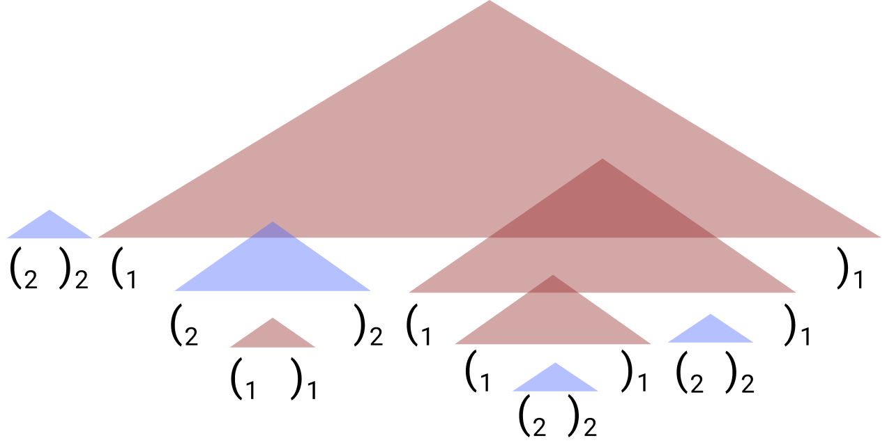
In this section we introduce the language we’ll work with: Dyck-$(k,m)$. We start with Dyck-$k$, the language of well-nested brackets of $k$ types. Like how there’s hierarchical structure in language, as in this example highlighting the relationships between subjects and verbs in center-embedded clauses:

There’s also hierarchical structure in Dyck-$k$, as in the following:

In fact, despite the simplicity of Dyck-$k$, in a strong sense it’s a prototypical language of hierarchical structure. Thinking back to the context-free languages, like those describable by constituency grammars, it turns out that Dyck-$k$ is at the core of all of these languages. This is formalized in the Chomsky-Schützenberger Theorem.

The connection that we’ve discussed between hierarchy and stacks is immediate in Dyck-$k$: upon seeing an open bracket of type $i$, memory of that bracket must be pushed onto a stack; upon seeing its corresponding close bracket of type $i$, it is popped.

But consider the fragment Laws the lawmaker the reporter questions writes are, from the example above. Isn’t it a little… hard to read? If you take a second, you can work out that the reporter is questioning a lawmaker, who writes laws, and those laws are the subject of the sentence. But consider the following sentence:

I found this one easier to read. Part of the reason for this is that the first sentence has nested center-embedded clauses, which require you to keep a bunch of memory around to know how subjects pair with verbs. The second one isn’t as deeply nested; you have to keep Laws around for a while before seeing are, but you only need to keep two items around (Laws, the lawmaker ) before you see wrote and can sort of relegate the lawmaker to less precise memory.

There’s a connection between this center-embedding depth and the depth of stack you need in order to parse sentences.⁷ Intuitively, it’s about the amount of memory you need in order to figure out the meaning. You only have so much working memory, and things get hard to understand when they test your limits. Dyck-$k$ can be arbitrarily deeply nested, but human language rarely goes deeper than center-embedding depth 3.⁸

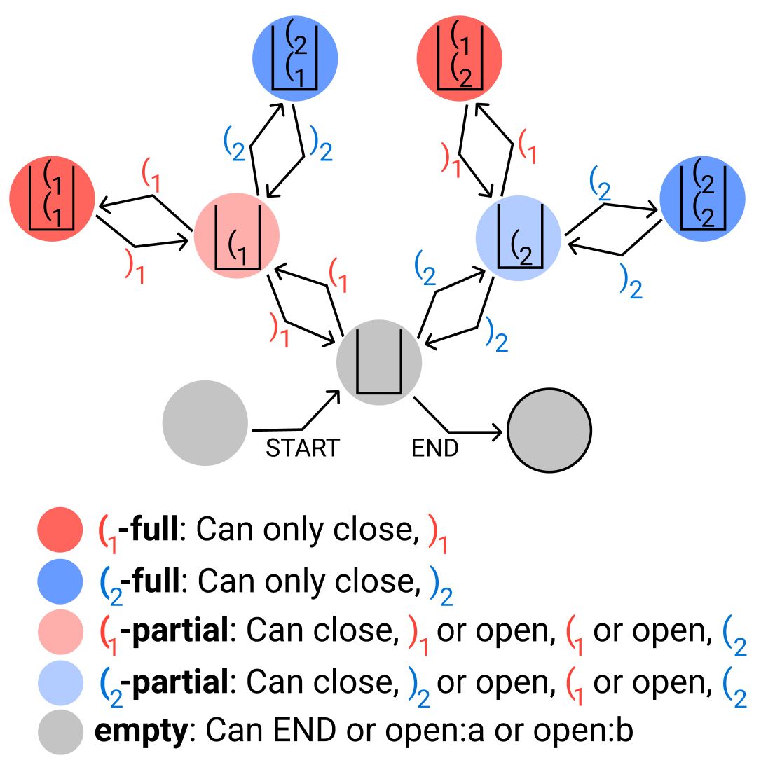
So, instead of studying RNNs’ ability to generate Dyck-$k$, we put a bound on the maximum depth of the stack of brackets, call it $m$, and call it Dyck-$(k,m)$. If you’re a fan of the Chomsky Hierarchy (regular languages, context-free, context-senstive, recursively enumerable), this means that Dyck-$(k,m)$ is a regular language, and so is recognizable by a finite-state machine (DFA). But it’s a regular language with special, stack-like states, like in the following example for Dyck-$(2,2)$:

Setting the focus on memory efficiency

Under our finite-precision setting, it’s a known result that for any regular language, you can take the minimal deterministic finite state machine, and encode that machine in the RNN using finite precision. So it may seem confusing at first why we’re asking new theoretical questions about RNNs and their ability to generate Dyck-$(k,m)$.

It’s because using those encodings of DFAs in RNNs, we’d need about $k^{m+1}$ hidden units in our RNNs in order to generate Dyck-$(k,m)$. This is a lot; think about $k=\mathrm{100,000}$ as the vocabulary size and $m=3$ as the stack depth; we’d need ${\mathrm{100,000}}^4={10}^{20}$ hidden units! Using our construction for the LSTM, we’d need $3m\lceil \log k\rceil -m=150$ hidden units.

Building a bounded stack using an extended model

Recall the Simple RNN equation,

$$h_t=\sigma (W{h}_{t-1}+U{x}_t+b)$$

We’ll now go into how you could build a bounded stack in an RNN, starting with an extended model that can do things popular RNNs can’t do, for ease of explanation. Our extended model is second-order RNNs, which can choose from recurrent matrices $W_x$ depending on which input you see.

Consider encoding a stack of up to $m$ elements, each of dimensionality $k$, using a $km$-dimensional vector:

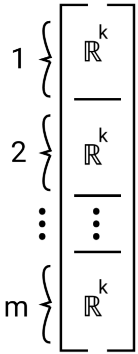
Think of each of the $k$ possible bracket types as being represented by one of $k$ one-hot vectors. We’d like the top of the stack to be in slot $1$. So when we push an element, we’ll write it directly to slot $1$. Whatever was in slot $1$, we want to shift away from slot $1$ to make room, which we can do with a matrix $W_{\text{push}}$, as follows:

Notice how, if we had $m$ elements on the stack already, the last one would be shifted off the hidden state. Next, if we’d like to pop the top element from the stack, this is easy enough with a separate matrix $W_{\text{pop}}$, as follows:

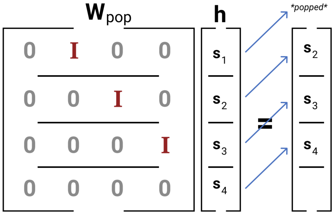
This works for our second-order RNN because if we see an open bracket, we can choose to apply $W_{\text{push}}$ to make room for it at the top, and if we see a close bracket, we can choose to apply $W_{\text{pop}}$ to forget its corresponding open bracket.

Why doesn’t this work for the Simple RNN that people use in practice? Because it only has one $W$ matrix, and for that matter, the LSTM does as well. So we’ll need to get a bit clever.

RNN stacks through push/pop subcomponents

We’ll get around the fact that there’s only one $W$ matrix by using a factor of $2$ more space, that is ,$2mk$ dimensions.

This corresponds to two $mk$-sized places where the stack could be stored. We’ll call one of them $h_{\text{pop}}$ and the other $h_{\text{push}}$, meaning where we write the stack when we apply a pop, and where we write the stack when we apply a push. Whichever place we don’t write the stack we’ll make sure is empty (that is, equals 0).

With these guarantees, we can read from both $h_{\text{pop}}$ and $h_{\text{push}}$ at once using a single $W$ matrix. By stacking $W_{\text{push}}$ and $W_{\text{pop}}$ matrices, we can do this, and use the same matrix to write to both $h_{\text{pop}}$ and $h_{\text{push}}$ what would happen if we saw each of pop or push:

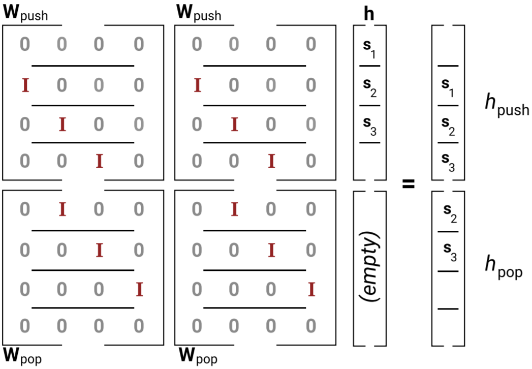
So looking at $Wh$, we’ve read from both $h_{\text{pop}}$ and $h_{\text{push}}$ and written to both as well. But we don’t want to write to both; we’d need only the one of $h_{\text{pop}}$ or $h_{\text{push}}$ that corresponds to the input we actually saw. For this we use the $U{x}_t$ term. Intuitively, when $x_t$ is an open bracket, $U{x}_t$ adds a very negative value to $h_{\text{pop}}$, which after the $\sigma$ nonlinearity results in $0$ values. When $x_t$ is a close bracket, $U{x}_t$ does the same thing, but for $h_{\text{push}}$. So, with $Wh+U{x}_t$, we’ve ensured that only one of $h_{\text{pop}}$ or $h_{\text{push}}$ is written to, and we read from both of them.

There you have it! It took an extra factor-$2$ of memory, but it’s an exact way to push or pop from a bounded-depth stack in an RNN.

LSTM stacks through clever gating

LSTMs were proposed to improve learning, solving the vanishing gradient problem of RNNs. Again we’re considering expressivity in this work, not learning, so we study whether the extra gating functions in LSTMs allow them to implement stacks more efficiently.

We find that yes, though we needed $2mk$ to implement our stack with the Simple RNN, we need $mk$ (like for second-order RNNs) for LSTMs, a factor-two improvement. Interestingly, the mechanism by which we prove this is completely separate from the push/pop components we used in the Simple RNN; instead, it relies entirely on the LSTM’s gates.

A quick glance at the memory dynamics

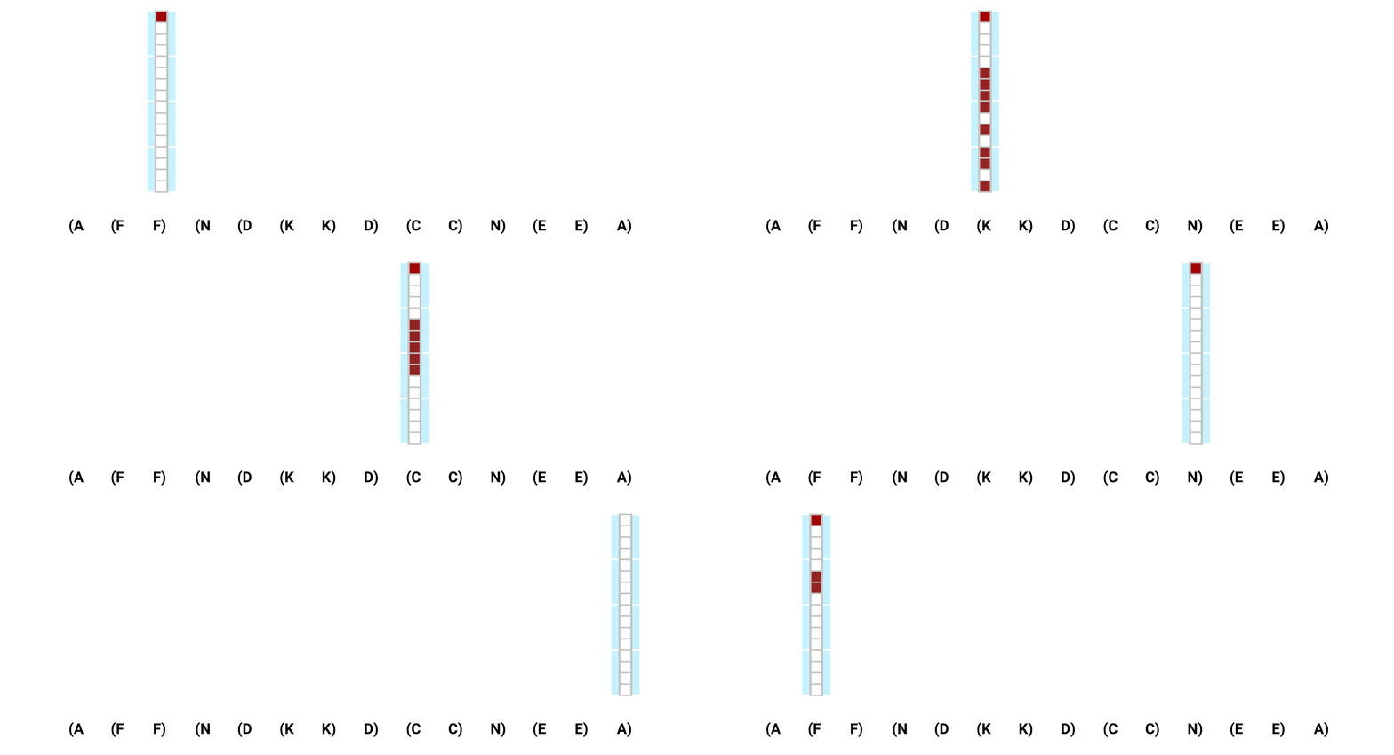
The exact mechanisms by which the constructions work are a bit involved, so we sketch out the main ideas here. Let’s start by walking through an example of how the LSTM’s memory behaves as it processes a sequence.

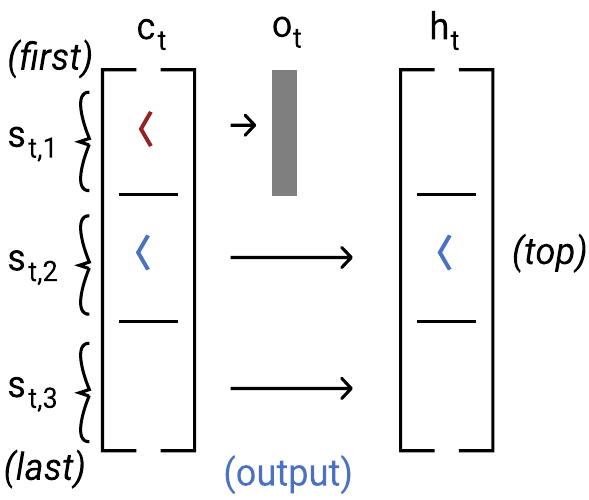
As is clear from the figure, the top of our LSTM’s stack isn’t always slot 1 like in the Simple RNN construction. Instead, the top of the stack is always the farthest non-empty slot from slot 1, and the bottom of the stack is slot 1. All brackets currently on the stack are stored in the cell state $c_t$, but only the top element of the stack is allowed through the output gate into the hidden state, $h_t$. This is visualized in the above diagram as the state that is shaded grey.

Recall the LSTM equations, or skip past them if you’d prefer, and remember that the LSTM has an input gate, an output gate, a forget gate, and a new cell candidate:

$$i_t=\sigma (W_i{h}_{t-1}+U_i{x}_t+b_i)$$$$o_t=\sigma (W_o{h}_{t-1}+U_o{x}_t+b_o)$$$$f_t=\sigma (W_f{h}_{t-1}+U_f{x}_t+b_f)$$$${\tilde{c}}_t=\text{tanh}(W_{\tilde{c}}{h}_{t-1}+U_{\tilde{c}}{x}_t+b_{\tilde{c}})$$$$c_t=i_t\cdot {\tilde{c}}_t+f_t\cdot c_{t-1}$$$$h_t=o_t\cdot \text{tanh}\left(c_t\right)$$

Intuitively, the input gate determines what new content (from ${\tilde{c}}_t$) is added to the memory cell $c_t$, and what old content (from $c_{t-1}$) is copied into the memory cell $c_t$. The output gate $o_t$ determines what information flows from the cell $c_t$ to the hidden state $h_t$.

Let’s go through how each of the gates contributes to the memory management that we saw in our example. We’ll discuss the behavior of each gate under each of the two stack operations: push and pop.

New cell candidate

To implement a push, the new cell candidate ${\tilde{c}}_t$ has the job of attempting to write an open bracket to the top of the stack. This is a bit difficult because, as we’ve said, the location where the new top of the stack should be written could be at any of the $m$ slots of the memory. Thus, the new cell candidate, through $U_{{\tilde{c}}^{}}{x}_t$ actually tries to write the identity of the bracket specified by $x_t$ to all m stack slots. This works because the new cell candidate relies on the input gate being $1$ only for the stack slot where the new element should be written, and $0$ elsewhere, so all other slots are unaffected.

To implement a pop, the new cell candidate does nothing! Its value is ${\tilde{c}}_t=0$ for any close bracket.

Input gate

To implement a push, the input gate $i_t$ has the job of deciding where the new element should be written, that is, where the new top of the stack will be. This is relatively easy; the input gate has access to the old hidden state through $W_i{h}_{t-1}$, and so it can detect the slot that was the top, and set itself to $1$ for the next. How does $W_i{h}_{t-1}$ figure that out? For the details, you’ll have to look to the appendix of our paper, or our PyTorch implementation, but here’s an idea. The $W_i$ matrix looks like this, as a block matrix, along with the bias term and an example hidden state that might be multiplied with it:

$$W_i=\left[\begin{array}{cccccc}-1& -1& -1& -1& -1& \cdots \\ 1& -1& 0& 0& 0& \cdots \\ 0& 1& -1& 0& 0& \cdots \\ 0& 0& 1& -1& 0& \cdots \\ 0& 0& 0& -1& 1& \cdots \\ ⋮& ⋮& ⋮& ⋮& ⋮& \ddots \end{array}\right]b_i=\left[\begin{array}{c}0.5\\ -1.5\\ -1.5\\ -1.5\\ -1.5\\ ⋮\end{array}\right]$$

$$h_{t-1}=\lceil$$$$\lfloor \begin{array}{c}0\\ 0\\ e_i\\ 0\\ 0\\ 0\end{array}]$$

(Where $e_i$ is the one-hot vector at index $i$). This is an informal way to describe the matrix, but consider each row and column as referring to a slot ($k$ dimensions). The hidden state from the last timestep $h_{t-1}$ encodes a bracket in slot $3$, so that’s where the top of the stack is. So the quantity $W_i{h}_{t-1}$ looks like $[-1,0,1,-1,0,\dots ]$. This means for slot $1$, the input to the sigmoid $\sigma \left(\right)$ for the input gate is $-1$ (from $W_i{h}_{t-1}$) plus the bias term $-0.5$, plus $1$ from the fact that an open bracket is seen (not shown in the diagram.) So the total input is $-1-0.5+1=-0.5$. By scaling the weights of all parameters to be large, we can make this $-0.5$ very large and negative, causing the input gate to equal $0$. This block of rows of the matrix effectively detects if any slot in the hidden state is non-zero, ensuring that the first slot is not written to in that case.

In this example, the new top of the stack should be written to slot $4$ (since the top is currently at slot $3$.) The contribution from $W_i{h}_{t-1}$ to the input gate of slot $4$ is $1$, summed with the bias term of $-1.5$ and the input contribution of $1$ because of the open bracket, for a sum of $0.5$. As before, by scaling all parameters to be large, we can cause this $0.5$ to become large, so the input gate saturates to $1$.

Now that we’ve gone through this example in some detail, we won’t for the other gates, but the stories are all similar: by carefull setting of the $W,U,b$ parameters, exact conditions can be tested for by each of the gates.

Here’s a diagram that summarizes the push operation:

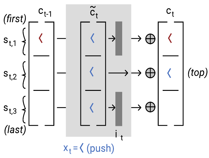
To implement a pop, the input gate doesn’t matter, since the new cell candidate is set to $0$.

Forget gate

To implement a push, the forget gate is set to $1$ everywhere, since all elements from the previous state should be remembered.

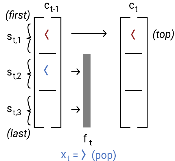
To implement a pop, the forget gate needs to detect where the top of the stack is, and be $0$ there, while ensuring that it is $1$ for all other slots that encode an element. This is accomplished, informally, by using $W_f$ to detect the only slot in $h_{t-1}$ that is non-zero; this is guaranteed to encode the top of the stack.

Here’s a diagram that summarizes the pop operation:

Output gate

The output gate determines where the top of the stack in $c_t$ is, and only lets that slot (out of all the non-zero slots) through to the hidden state $h_t$. This is tricky, since the output gate equations don’t refer to $c_t$; they only refer to $h_{t-1}$ and $x_t$. However, breaking the possible situations into cases (where the top of the stack was, and whether $x_t$ pushes or pops an element), we show that the output gate can operate as required, just letting the top of the stack through, as visualized in this diagram:

With that, we’ve informally described the entire mechanism of the LSTM construction. For more detail, take a look at our paper, or play around with our PyTorch implementation, which actually prints out the valus of the gates at each timestep.

A distributed vocabulary code

So far, we’ve considered encoding a stack of up to $m$ elements from a universe of size $k$ using $km$ many dimensions, but our theoretical claim is that we can get away with $O\left(m\log k\right)$ dimensions. The only key insight left is to develop an efficient encoding of $k$ vocabulary items in $O\left(\log k\right)$ space such that (1) the identity of the bracket is linearly decodable (remember we’re making a language model, and we’ve only got one layer!) and (2) such that the stack mechanisms all still work.

A naive attempt is to assign each of the $k$ bracket types one of the $2^{{\log }_{2}k}$ many configurations of a $\log k$-dimensional binary vector, which we’ll call $p_i$ for bracket $i$. This doesn’t obey constraint (1); since some encodings (like $\left[1111\right]$) are supersets of others (like $\left[0001\right]$), so trying to read out the subset vector will never assign more probability to the subset than the superset.

We can get away from this by adding a constant factor more space and concatenating the binary negation $(1-p_i)$, so that now each stack slot takes $2\lceil {\log }_{2}k\rceil$ space. When attempting to read out element $i$, we can use the encoding of $i$ itself, since for any two encodings ${\varphi }_i,{\varphi }_j$, the dot product between their representations is

$${\varphi }_i^{\top }{\varphi }_j=\sum _{\ell =1}^{\lceil \log k\rceil }{\varphi }_{i,\ell }^{\top }{\varphi }_{j\ell }+\sum _{\ell =1}^{\lceil \log k\rceil }(1-ph{i}_{i,\ell }{)}^{\top }(1-{\varphi }_{j\ell })$$

This quantity is equal to $\lceil \log k\rceil$ if $i=j$, and is strictly less otherwise; it effectively checks if each dimension agrees.

We won’t go into how the stack constructions are guaranteed to work (constraint 2), but we end up needing a constant factor more space, and with a few other details we end up with $3m\lceil \log k\rceil -m$ hidden units sufficient for the LSTM, and $6m\lceil \log k\rceil -2m$ hidden units sufficient for the Simple RNN.

A matching lower-bound

So, is $O\left(m\log k\right)$ a “good” number of hidden units for generating Dyck-$(k,m)$? Turns out, it’s great. (And look at the constants; they’re not so bad either!) In fact, nothing that uses a vector memory could do better than $O\left(m\log k\right)$ dimensions, which we can prove with a simple communication complexity argument.

There are at least $k^m$ distinct strings that any algorithm that generates Dyck-$(k,m)$ must distinguish in its memory. (Think about any input that lists $m$ open brackets to start – these must all be assigned different representations.) With $p=O\left(1\right)$ bits of precision to represent each of $d$ dimensions of a vector, there are exactly $2^{dp}$ possible configurations that the vector can take on. Combining these facts, we get that we need $2^{dp}\ge k^m$, and so $d=\frac{m\log k}{p}=O\left(m\log k\right)$.

That’s it!

Bonus: some experiments

We’ve focused on what RNNs can express, not what they learn. But take a look at this plot, where we’ve trained LSTM LMs (with hidden state sizes provided by our theory) on samples Dyck-$(k,m)$ for various values of $k$ and $m$ and training set sizes, and tested them on longer sequences than those seen at training time.

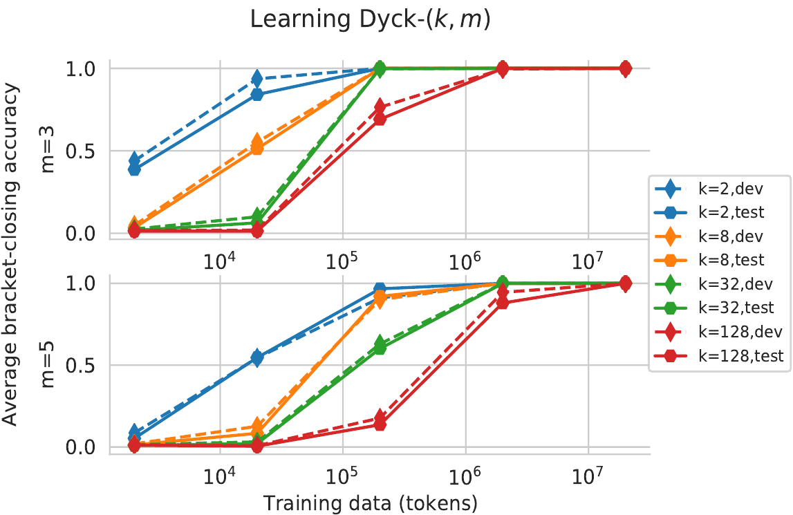
With enough training data, all of the networks achieved less than ${10}^{-4}$ error (on a metric that measures whether brackets are predicted correctly). Perhaps surprisingly, this is despite the fact that for large values of $k$, a vanishingly small percent of the possible stack states (sequences of unclosed open brackets) are seen at training time. Unseen stack states at test time are handled, showing that the LSTM doesn’t simply learn $k^{m+1}$ structureless DFA states, but instead may be exhibiting stack-like behavior.

Concluding thoughts

What a ride it’s been.

I was surprised that RNNs in this finite-precision setting could implement the operations of a stack—as long as you don’t require unbounded memory of it—and I was more surprised that it can do so optimally memory-efficiently. We see this as an argument that neural networks’ expressivity shouldn’t (only) be cast in terms of the Chomsky Hierarchy, which relegates all finite-memory languages to the regular category. Here, we saw that because of the special, stack-like structure of Dyck-$(k,m)$, RNNs could generate it exponentially more efficiently than you might expect. So, it’s the structure of the language, and the structure of the hidden state space, that’s really interesting.

I hope this work inspires ways to think about how RNNs work, how to analyze them, and how to build architectures that better learn how to process hierarchical structure.

Footnotes